8.1.2 Explore Univariae Distributions of the Variables
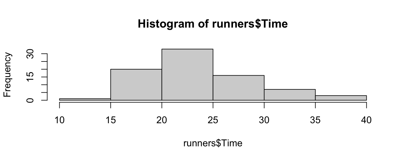
hist(runners$Time)
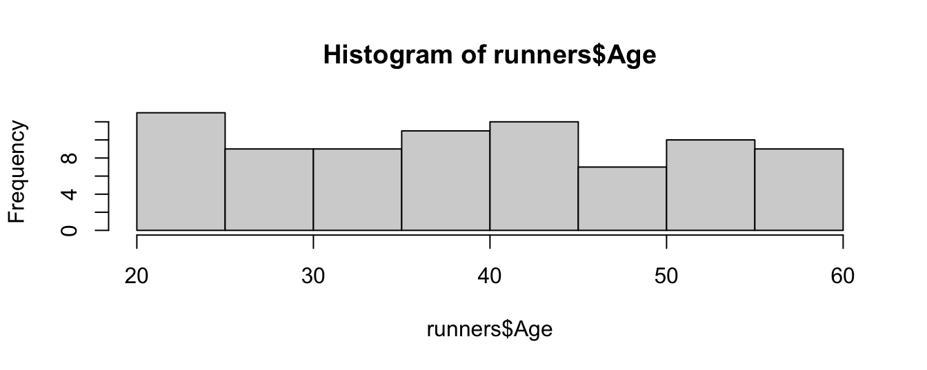
hist(runners$Age)
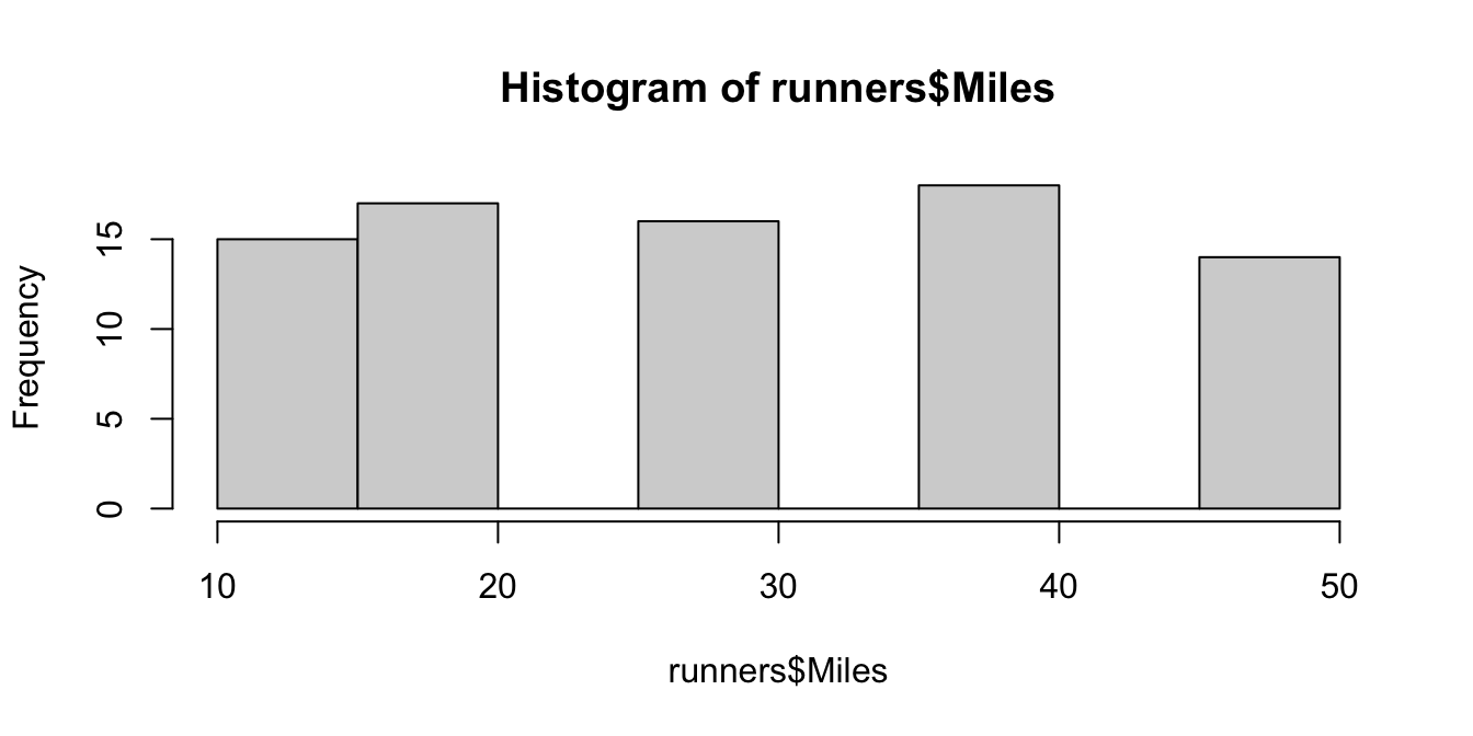
hist(runners$Miles)
describe(runners, fast =TRUE)
      vars  n  mean    sd median   min   max range  skew kurtosis   se
Time     1 80 23.55  5.29   22.9 14.87 37.75 22.88  0.64    -0.14 0.59
Age      2 80 39.66 11.56   39.0 20.00 59.00 39.00  0.07    -1.24 1.29
Miles    3 80 29.88 13.82   30.0 10.00 50.00 40.00 -0.01    -1.29 1.55
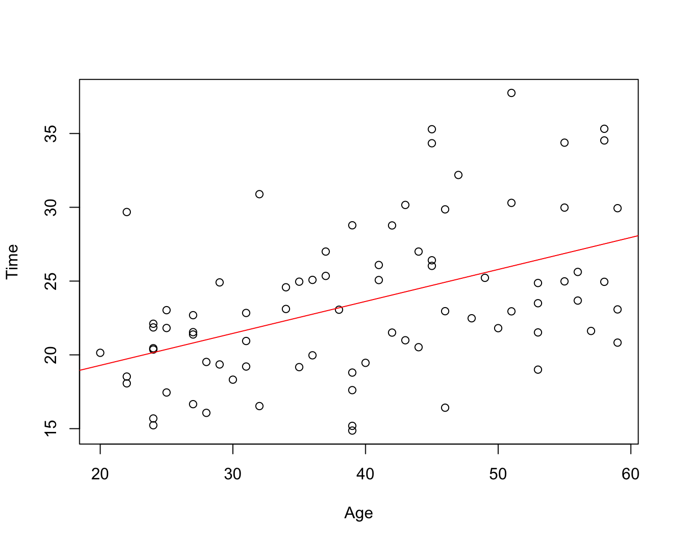
8.1.3 Visualize the Bivariate Relations Between Variables
plot(Time ~ Age, runners)abline(reg =lm(Time ~ Age, runners), col ="red")
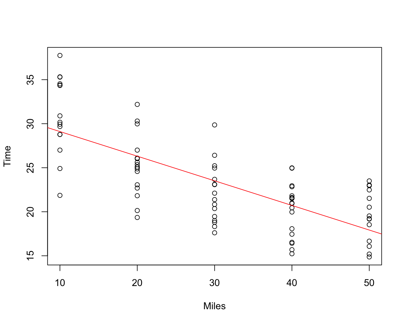
plot(Time ~ Miles, runners)abline(reg =lm(Time ~ Miles, runners), col ="red")
8.1.4 Quantifying Bivariate Relations
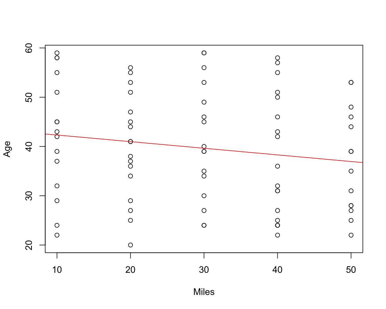
plot(Age ~ Miles, runners)abline(reg =lm(Age ~ Miles, runners), col ="red")
print(cor(runners), digits =2)
       Time   Age Miles
Time   1.00  0.47 -0.73
Age    0.47  1.00 -0.16
Miles -0.73 -0.16  1.00
8.1.5 Multiple Regression: Additive Model
additivemod <-lm(Time ~ Age + Miles, data = runners)summary(additivemod)
Call:
lm(formula = Time ~ Age + Miles, data = runners)

Residuals:
    Min      1Q  Median      3Q     Max
-6.7507 -2.3133  0.0271  2.2358  7.1882

Coefficients:
            Estimate Std. Error t value Pr(>|t|)
(Intercept) 24.60519    1.57309  15.641  < 2e-16 ***
Age          0.16724    0.03059   5.468 5.43e-07 ***
Miles       -0.25728    0.02558 -10.057 1.13e-15 ***
---
Signif. codes:  0 '***' 0.001 '**' 0.01 '*' 0.05 '.' 0.1 ' ' 1

Residual standard error: 3.103 on 77 degrees of freedom
Multiple R-squared:  0.6648,    Adjusted R-squared:  0.6561
F-statistic: 76.35 on 2 and 77 DF,  p-value: < 2.2e-16
8.1.9 Interpreting Coefficients in Models with Interactions
8.1.9.1 Additive Model
The coefficient is the expected change in the outcome (Y) for a one unit change in this predictor (X1) holding the other predictor (X2) constant
This effect of X1 is the same no matter what the value of X2
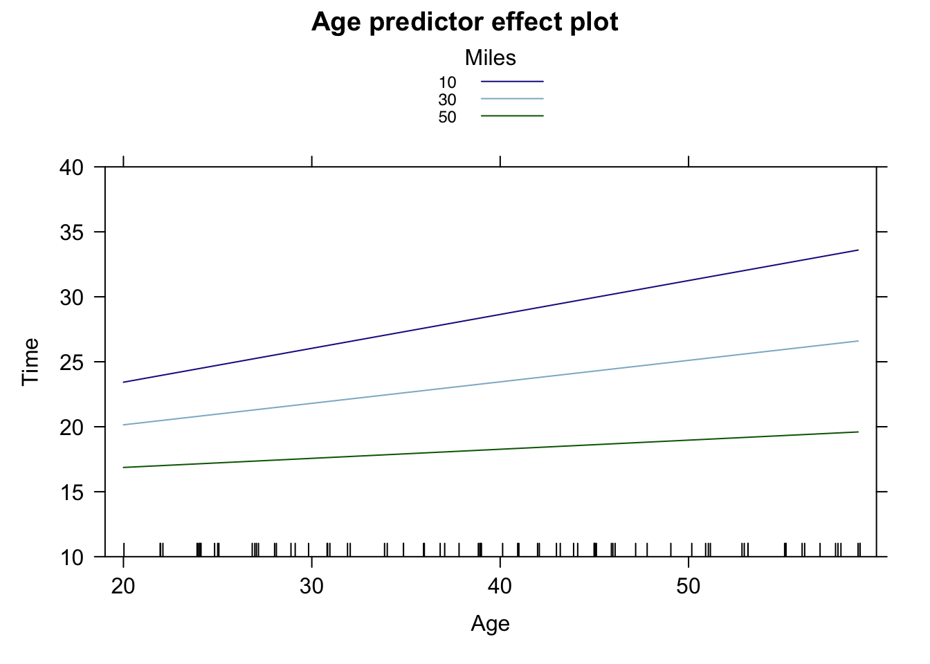
8.1.9.2 Moderation Model (with Interaction)
For variables included in the interaction term, the coefficient is interpreted as the effect of a one unit change in that predictor (X1) on the outcome (Y) when the other predictor in the interaction (X2) is zero.
The size of the effect of X1 on Y changes depending on the value of X2.