n <- 10000
mu <- 67
sigma <- 4

b0 <- 0
b1 <- 1

repht <- rnorm(n, b0, sigma)

height <- b0 + b1*repht + rnorm(n, 0, sigma)6 Multivariate Linear Models
6.1 Assumptions of Linear Models
Linearity - Expected value of the response variable is a linear function of the explanatory variables.
Constant Variance(Homogeneity of variance; Identically distributed) - The variance of the errors is constant across values of the explanatory variables.
Normality - The errors (residuals) are normally distributed, with an expected mean of zero (unbiased).
Independence - The observations are sampled independently (the residuals are independent).
No measurement error in predictors - The predictors are measured without error. THIS IS AN IMPORTANT AND ALMOST ALWAYS VIOLATED ASSUMPTION.
Predictors are not Invariant - No predictor is constant.
6.2 Review of Simple Regression with a Simulation
\[ Y_i = b_0 + b_1 X_i + e_i \]
\[ height_i = b_0 + b_1 repht_i + e_i \]
plot(height ~ repht, col = "grey")
abline(reg = lm(height ~ repht))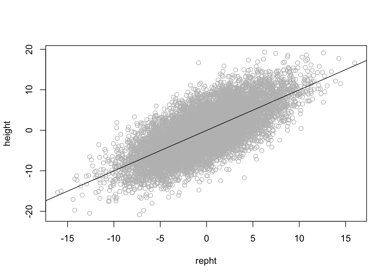
6.3 Simple Regression Model
mod.simple <- lm(height ~ repht)
summary(mod.simple)
Call:
lm(formula = height ~ repht)

Residuals:
     Min       1Q   Median       3Q      Max
-15.4079  -2.6550   0.0089   2.6378  14.7846

Coefficients:
            Estimate Std. Error t value Pr(>|t|)
(Intercept) -0.02558    0.03971  -0.644     0.52
repht        0.99586    0.00984 101.204   <2e-16 ***
---
Signif. codes:  0 '***' 0.001 '**' 0.01 '*' 0.05 '.' 0.1 ' ' 1

Residual standard error: 3.971 on 9998 degrees of freedom
Multiple R-squared:  0.506, Adjusted R-squared:  0.506
F-statistic: 1.024e+04 on 1 and 9998 DF,  p-value: < 2.2e-16
6.4 Plotting Residuals
plot(resid(mod.simple) ~ predict(mod.simple))
abline(h = 0, col = "red")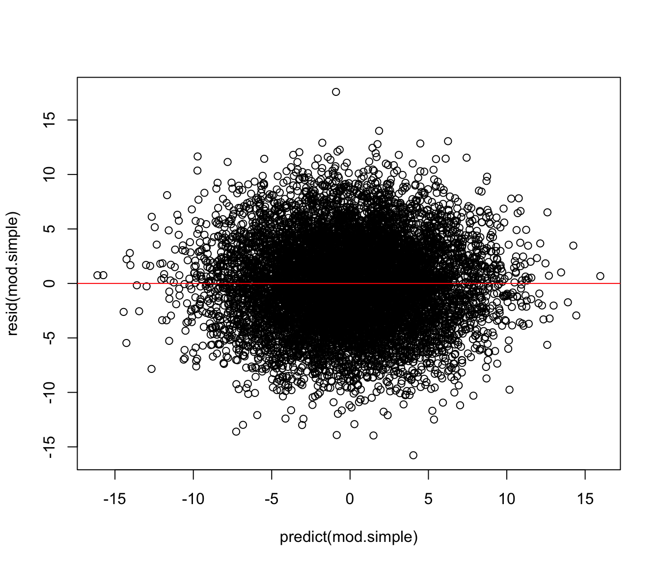
7 Multiple Regression
7.1 Weight Data from Chapter 6
mswt <- read.csv("data/middleschoolweight.csv", header = TRUE)
str(mswt)
'data.frame': 19 obs. of 5 variables:
$ Name : chr "Alfred" "Antonia" "Barbara" "Camella" ...
$ Sex : chr "M" "F" "F" "F" ...
$ Age : int 14 13 13 14 14 12 12 15 13 12 ...
$ Height: num 69 56.5 65.3 62.8 63.5 57.3 59.8 62.5 62.5 59 ...
$ Weight: num 112 84 98 102 102 ...7.2 Look at some of the data
library(psych)
headTail(mswt) # in the psych package
Name Sex Age Height Weight
1 Alfred M 14 69 112.5
2 Antonia F 13 56.5 84
3 Barbara F 13 65.3 98
4 Camella F 14 62.8 102.5
... <NA> <NA> ... ... ...
16 Robert M 12 64.8 128
17 Sequan M 15 67 133
18 Thomas M 11 57.5 85
19 William M 15 66.5 1127.3 Visualizing Weight versus Height
library(car)
scatterplot(Weight ~ Height,
            data = mswt,
            regLine = FALSE,
            smooth = FALSE,
            id = list(labels = mswt$Name,
                      n = 2),
            boxplots = FALSE)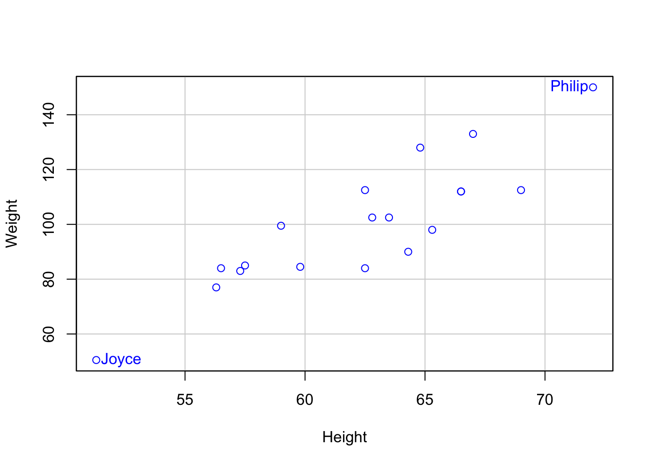
 Joyce Philip
    11     15
7.4 Visualizing Weight and Age
plot(Weight ~ Age, mswt)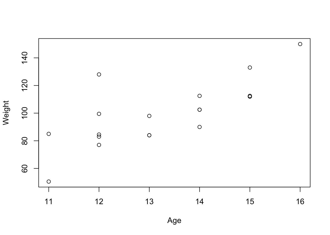
7.5 Scatterplot Matrix
pairs(mswt[ ,-(1:3)])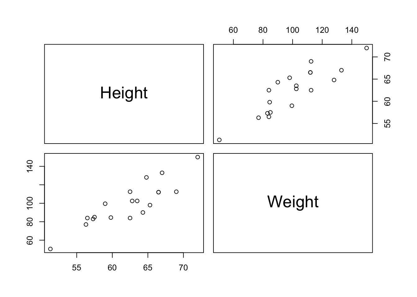
7.6 Descriptive Statistics
describe(mswt[ ,-(1:2)]) vars n mean sd median trimmed mad min max range skew kurtosis
Age 1 19 13.32 1.49 13.0 13.29 1.48 11.0 16 5.0 0.05 -1.33
Height 2 19 62.34 5.13 62.8 62.42 5.49 51.3 72 20.7 -0.22 -0.67
Weight 3 19 100.03 22.77 99.5 100.00 21.50 50.5 150 99.5 0.16 -0.11
se
Age 0.34
Height 1.18
Weight 5.227.7 Empty Model of Weight
mod0 <- lm(Weight ~ 1, data = mswt)
summary(mod0)
Call:
lm(formula = Weight ~ 1, data = mswt)

Residuals:
    Min      1Q  Median      3Q     Max
-49.526 -15.776  -0.526  12.224  49.974

Coefficients:
            Estimate Std. Error t value Pr(>|t|)
(Intercept)  100.026      5.225   19.14 2.05e-13 ***
---
Signif. codes:  0 '***' 0.001 '**' 0.01 '*' 0.05 '.' 0.1 ' ' 1

Residual standard error: 22.77 on 18 degrees of freedom
7.8 Model of Weight on Age
mod.height <- lm(Weight ~ Age, data = mswt)
summary(mod.height)
Call:
lm(formula = Weight ~ Age, data = mswt)

Residuals:
    Min      1Q  Median      3Q     Max
-23.349  -7.609  -5.260   7.945  42.847

Coefficients:
            Estimate Std. Error t value Pr(>|t|)
(Intercept)  -50.493     33.290  -1.517 0.147706
Age           11.304      2.485   4.548 0.000285 ***
---
Signif. codes:  0 '***' 0.001 '**' 0.01 '*' 0.05 '.' 0.1 ' ' 1

Residual standard error: 15.74 on 17 degrees of freedom
Multiple R-squared:  0.5489,    Adjusted R-squared:  0.5224
F-statistic: 20.69 on 1 and 17 DF,  p-value: 0.0002848
7.9 Centering the Predictor
mswt$cAge <- mswt$Age - mean(mswt$Age)
mod.cage <- lm(Weight ~ cAge, data = mswt)
summary(mod.cage)
Call:
lm(formula = Weight ~ cAge, data = mswt)

Residuals:
    Min      1Q  Median      3Q     Max
-23.349  -7.609  -5.260   7.945  42.847

Coefficients:
            Estimate Std. Error t value Pr(>|t|)
(Intercept)  100.026      3.611  27.702 1.38e-15 ***
cAge          11.304      2.485   4.548 0.000285 ***
---
Signif. codes:  0 '***' 0.001 '**' 0.01 '*' 0.05 '.' 0.1 ' ' 1

Residual standard error: 15.74 on 17 degrees of freedom
Multiple R-squared:  0.5489,    Adjusted R-squared:  0.5224
F-statistic: 20.69 on 1 and 17 DF,  p-value: 0.0002848
7.10 Basic Ideas
- simple regression analysis: 1 IV
\[Y_i = a + b_1 X_i + e_i\]
- multiple regression: 2 + IVs
\[Y_i = a + b_1 X_{1i} + b_2 X_{2i} + \dots + b_k X_{ki} + e_i\]
- to find \(b_k\) (i.e., \(b_1, b_2, \dots, b_k\)) so that \(\Sigma{e^2}\) [i.e. \(\Sigma (Y - \hat{Y})^2\)] is minimal (least squares principle).
7.11 Four Reasons for Conducting Multiple Regression Analysis
To explain how much variance in \(Y\) can be accounted for by \(X_1\) and \(X_2\). For example, how much variation in Reading Achievement ( \(Y\) ) can be accounted for by Verbal Aptitude( \(X_1\) ) and Achievement Motivation ( \(X_2\) )?
To test whether the obtained sample regression coefficients (\(b_1\) an \(b_2\)) are statistically different from zero. For example, is it reasonable that these sample coefficients have occurred due to sampling error alone (“by chance”)?
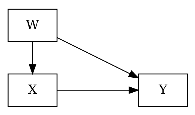
Illustration of an added independent variable ( \(X_3\) ) explains additional variance in \(Y\) above the other regressors.
To evaluate the relative importance of the independent variables in explaining variation in \(Y\).
7.12 Obtaining Simple and Multiple Regression Models
Give this a try
7.12.1 R code
exercise <- read.csv("data/exercise.csv", header = TRUE)
mod_exer <- lm(wtloss ~ exercise, data = exercise)
mod_food <- lm(wtloss ~ food, data = exercise)
mod_exer_food <- lm(wtloss ~ exercise + food,
                    data = exercise)
7.13 Comparing Simple and Multiple Regression Models
library(texreg)
htmlreg(list(mod_exer, mod_food, mod_exer_food), doctype = FALSE,
          custom.model.names = c("exercise", "food", "both"),
caption = "Models Predicting Weight Loss")| exercise | food | both | |
|---|---|---|---|
| (Intercept) | 4.00** | 7.14* | 6.00** |
| (0.91) | (2.92) | (1.27) | |
| exercise | 1.75** | 2.00*** | |
| (0.36) | (0.33) | ||
| food | 0.07 | -0.50 | |
| (0.54) | (0.25) | ||
| R2 | 0.75 | 0.00 | 0.84 |
| Adj. R2 | 0.71 | -0.12 | 0.79 |
| Num. obs. | 10 | 10 | 10 |
| ***p < 0.001; **p < 0.01; *p < 0.05 | |||
7.13.1 Raw Regression Coefficients ( \(b\)s ) vs Standardized Regression Coefficients ( \(\beta\)s )
- As if things were not confusing enough, \(\beta\), in addition to representing the population parameter, is also often used to represent the standardized regression coefficient
7.14 Relationship Between \(b\) and \(\beta\)
\(b_k = \beta_k \frac{s_y}{s_k}\), where \(k\) indicates the \(k\)th IV \(X_k\) and \(s\) is the standard deviation.
\(\beta_k = b_k \frac{s_k}{s_y}\)
With 1 IV, \(\beta = r_{xy}\)
7.15 Standardized Coefficients in R
library(parameters)
parameters(mod_exer_food, standardize = "smart")
Parameter | Std. Coef. | SE | 95% CI | t(7) | p
----------------------------------------------------------------
(Intercept) | 0.00 | 0.00 | [ 0.00, 0.00] | 4.71 | 0.002
exercise | 0.99 | 0.16 | [ 0.60, 1.38] | 6.00 | < .001
food | -0.33 | 0.16 | [-0.72, 0.06] | -1.98 | 0.088 7.16 Standardized Coefficients in R
zmod_exer_food <- lm(scale(wtloss) ~ scale(exercise) +
                     scale(food),
                     data = exercise)
print(summary(zmod_exer_food), digits = 5)
Call:
lm(formula = scale(wtloss) ~ scale(exercise) + scale(food), data = exercise)

Residuals:
     Min       1Q   Median       3Q      Max
-0.60455 -0.30228  0.00000  0.30228  0.60455

Coefficients:
                   Estimate  Std. Error t value  Pr(>|t|)
(Intercept)      7.1031e-18  1.4452e-01  0.0000 1.0000000
scale(exercise)  9.8723e-01  1.6454e-01  6.0000 0.0005423 ***
scale(food)     -3.2649e-01  1.6454e-01 -1.9843 0.0876228 .
---
Signif. codes:  0 '***' 0.001 '**' 0.01 '*' 0.05 '.' 0.1 ' ' 1

Residual standard error: 0.457 on 7 degrees of freedom
Multiple R-squared:  0.83756,   Adjusted R-squared:  0.79115
F-statistic: 18.047 on 2 and 7 DF,  p-value: 0.0017274
7.17 Unstandardized and Standardized Coefficients
7.18 Basic Ideas: \(R^2\)
\[ Y_i = a + b_1 X_i + e_i \]
\(r^2_{yx}\) is the proportion of variance in \(Y\) accounted for by \(X\).
\[Y_i = a + b_1 X_{1i} + b_2 X_{2i} + e_i\]
\(r^2_{y12} = r^2_{\hat{Y}Y} = R^2\) is the proportion of variance in \(Y\) accounted for by \(X_1\) and \(X_2\) combined
when \(r_{12} = 0, \quad r^2_{y12} = r^2_{y1} + r^2_{y2}\)
when \(r^2_{12} \neq 0\), see next slide
7.19 \(R^2\) Represented Graphically
#include_graphics("products/slides/figures/venn.jpg")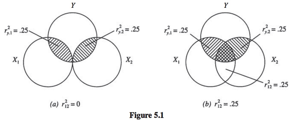
7.21 Squared Multiple Correlation Coefficient
\[R^2 = \frac{SS_{reg}}{SS_{total}}\]
\[R^2 = r^2_{Y,\hat{Y}}\]
\[R^2 = \frac{r^2_{y1} + r^2_{y2} - 2r_{y1}r_{y2}r_{12}}{1 - r^2_{12}}\]
when \(r_{12} = 0\): \(R^2 = r^2_{y1} + r^2_{y2}\)
7.22 Tests of Significance and Interpretation
7.22.1 Test of \(R^2\)
\[F_{(df1, df2)} = \frac{R^2/k}{(1 - R^2)/(N - k - 1)}, \quad df_1 = k, df_2 = N - k - 1.\]
7.22.2 Test of \(SS_{reg}\)
\[F_{(df1, df2)} = \frac{SS_{reg}/k}{SS_{error}/(N - k - 1)}, \quad df_1 = k, df_2 = N - k - 1.\]
7.23 Tests of Significance and Interpretation
in simple regression analysis, test for the only regression coefficient \(b\) is the same as the test of \(R^2\) and the same as test of \(SS_{reg}\).
in multiple regression analysis, test of \(R^2\) and test of \(SS_{reg}\) is a test of all regression coefficients simultaneously.
in multiple regression analysis, the test of individual regression coefficient \(b_k\) is testing the unique contribution of \(X_k\), given all other independent variables are already in the model (contribution of \(X_k\) over and beyond other independent variables).
7.24 Relative Importance of Predictors
- the magnitude of \(b_k\) is affected by the scale of measurement
- NOT ideal for inferring substantive or statistical meaningfulness
- NOT ideal for inferring relative importance across variables in model
- for different populations, can be used for assessing the importance of the same variable across populations.
- \(\beta\) is on a standardized scale (in standard deviation units: a \(z\) score)
- better for assessing relative importance across variables in model (though we will find that there are problems with this)
- magnitude impacted by group \(s\), thus less suitable for comparisons across populations.
8 Divorce Example
library(rethinking)
data("WaffleDivorce")
divorce <- WaffleDivorce
rm(WaffleDivorce)
divorce$whm <- divorce$WaffleHouses/divorce$Population
8.1 Waffle Houses and Divorce Rates
ggplot(divorce, aes(whm, Divorce)) + geom_point() +
  geom_text(aes(label = ifelse(Divorce > 11 | WaffleHouses > 70, as.character(Loc), '' )), hjust = -.3, vjust = -.3) +
  geom_smooth(method = "lm") +
  xlab("Waffle Houses per million") + ylab("Divorce rate")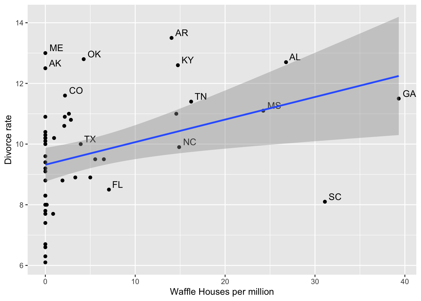
8.2 Waffle Houses and Divorce Rates: Simple Regression Table
mod <- lm(Divorce ~ whm, data = divorce)
htmlreg(mod, custom.coef.names = c("(Intercept", "Waffle houses/million"), doctype = FALSE,
custom.model.names = "Simple Regression")| Simple Regression | |
|---|---|
| (Intercept | 9.32*** |
| (0.28) | |
| Waffle houses/million | 0.07** |
| (0.03) | |
| R2 | 0.13 |
| Adj. R2 | 0.12 |
| Num. obs. | 50 |
| ***p < 0.001; **p < 0.01; *p < 0.05 | |
8.3 Spurious Association
| ## Divorce and Marriage |
|---|
| Variable M SD 1 2 |
     1. c1read      36.40    9.80


     2. c1genk      24.03    7.40 .49**

                                  [.47, .51]


     3. c5read     133.39   26.21 .53**        .61**

                                  [.52, .55]   [.59, .62]
Table: Real data
8.4 ECLSK simulated data
pandoc.table(tab2[[3]], caption = "Simulated data",
justify = c('left', 'left', 'right', 'right', 'left', 'left'))| Variable | M | SD | 1 | 2 | |
|---|---|---|---|---|---|
| 1. c1read | 36.40 | 9.81 | |||
| 2. c1genk | 23.98 | 7.38 | .49** | ||
| [.47, .51] | |||||
| 3. c5read | 133.00 | 26.34 | .54** | .61** | |
| [.52, .55] | [.59, .62] |
8.5 Title
g1 <- ggplot(ach3, aes(c1read, c5read)) +
  geom_point(alpha = .4) +
  theme(legend.position = "none") +
  # geom_smooth(method = "lm", fullrange = TRUE) +
  ylim(40, 250) + xlim(-10, 130) +
  ggtitle("k Reading and 5th Reading")
      g2 <- ggplot(ach3, aes(c1genk, c5read)) +
  geom_point(alpha = .4) +
  theme(legend.position = "none") +
  # geom_smooth(method = "lm", fullrange = TRUE) +
  ylim(40, 250) + xlim(-10, 130) +
  ggtitle("k General Know. and 5th Reading")

grid.arrange(g1, g2, nrow = 1)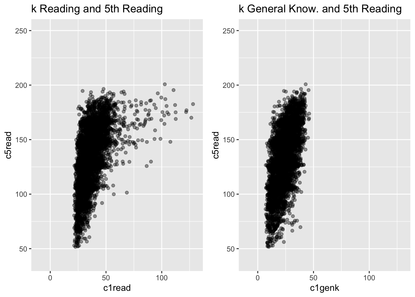
8.6 Three Models
rmodread <- lm(c5read ~ c1read, ach3)
rmodgenk <- lm(c5read ~ c1genk, ach3)
rmodML <- lm(c5read ~ c1read + c1genk, ach3)
htmlreg(list(rmodread, rmodgenk, rmodML), doctype = FALSE)| Model 1 | Model 2 | Model 3 | |
|---|---|---|---|
| (Intercept) | 81.42*** | 81.62*** | 64.28*** |
| (1.08) | (0.90) | (1.04) | |
| c1read | 1.43*** | 0.83*** | |
| (0.03) | (0.03) | ||
| c1genk | 2.15*** | 1.62*** | |
| (0.04) | (0.04) | ||
| R2 | 0.29 | 0.37 | 0.44 |
| Adj. R2 | 0.29 | 0.37 | 0.44 |
| Num. obs. | 6206 | 6206 | 6206 |
| ***p < 0.001; **p < 0.01; *p < 0.05 | |||
8.7 Comparing Real and Simulated Data
g1 <- ggplot(ach3, aes(c1read, c5read)) +
  geom_point(alpha = .4) +
  theme(legend.position = "none") +
  geom_smooth(method = "lm", fullrange = TRUE) +
  ylim(40, 250) + xlim(-10, 130) +
  ggtitle("Real Data")

g2 <- ggplot(simach3, aes(c1read, c5read)) +
  geom_point(alpha = .4) +
  theme(legend.position = "none") +
  geom_smooth(method = "lm", fullrange = TRUE) +
  ylim(40, 250) + xlim(-10, 130) +
  ggtitle("Simulated Data")

grid.arrange(g1, g2, nrow = 1)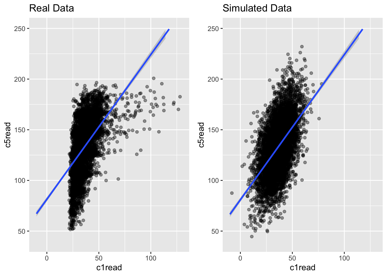
8.8 Comparing Real and Simulated Data
g1 <- ggplot(ach3, aes(c1genk, c5read)) +
  geom_point(alpha = .4) +
  theme(legend.position = "none") +
  geom_smooth(method = "lm", fullrange = TRUE) +
  ylim(40, 250) + xlim(-10, 130) +
  ggtitle("Real Data")

g2 <- ggplot(simach3, aes(c1genk, c5read)) +
  geom_point(alpha = .4) +
  theme(legend.position = "none") +
  geom_smooth(method = "lm", fullrange = TRUE) +
  ylim(40, 250) + xlim(-10, 130) +
  ggtitle("Simulated Data")

grid.arrange(g1, g2, nrow = 1)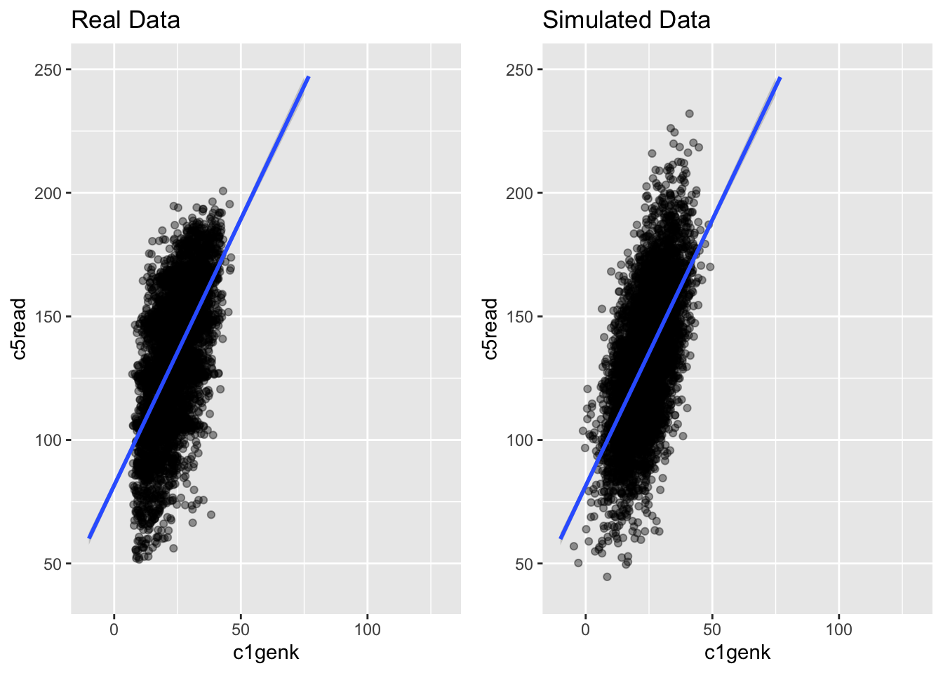
8.9 Comparing Real and Simulated Data
g1 <- ggplot(ach3, aes(c1read, c1genk)) +
  geom_point(alpha = .4) +
  theme(legend.position = "none") +
  geom_smooth(method = "lm", fullrange = TRUE) +
  ylim(-15, 50) + xlim(-10, 80) +
  ggtitle("Real Data")

g2 <- ggplot(simach3, aes(c1read, c1genk)) +
  geom_point(alpha = .4) +
  theme(legend.position = "none") +
  geom_smooth(method = "lm", fullrange = TRUE) +
  ylim(-15, 50) + xlim(-10, 80) +
  ggtitle("Simulated Data")

grid.arrange(g1, g2, nrow = 1)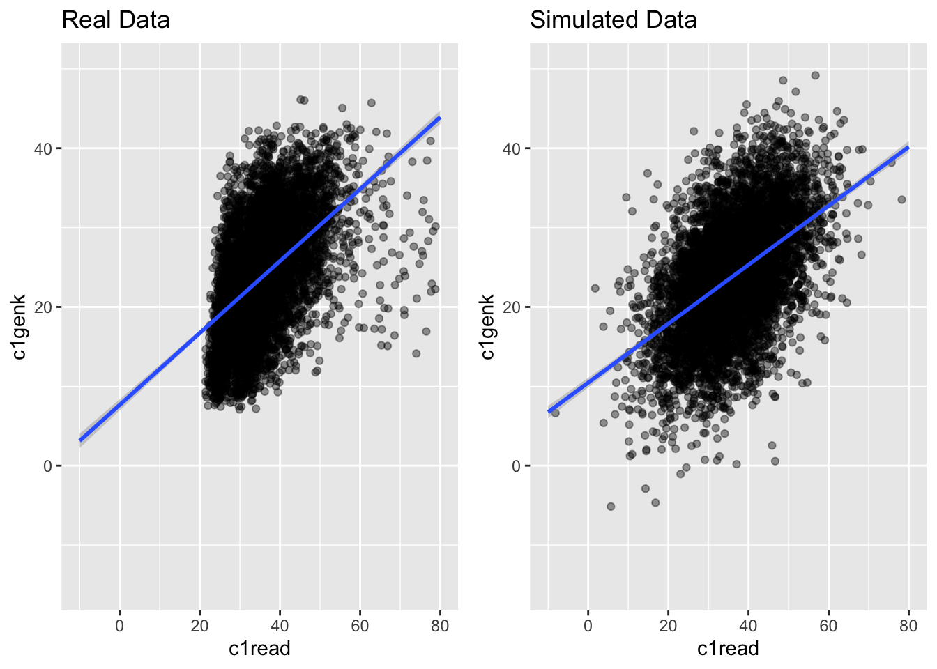
8.10 Comparing Two Simulated Data Sets
tab <- apaTables::apa.cor.table(data = simach3)
tab2 <- apaTables::apa.cor.table(data = simach3orthogonal)
pandoc.table(tab[[3]], caption = "Simulated data 1",
justify = c('left', 'left', 'right', 'right', 'left', 'left'))| Variable | M | SD | 1 | 2 | |
|---|---|---|---|---|---|
| 1. c1read | 36.40 | 9.81 | |||
| 2. c1genk | 23.98 | 7.38 | .49** | ||
| [.47, .51] | |||||
| 3. c5read | 133.00 | 26.34 | .54** | .61** | |
| [.52, .55] | [.59, .62] |
8.11 Comparing Two Simulated Data Sets
pandoc.table(tab2[[3]], caption = "Simulated data 2",
justify = c('left', 'left', 'right', 'right', 'left', 'left'))| Variable | M | SD | 1 | 2 | |
|---|---|---|---|---|---|
| 1. c1read | 36.62 | 9.80 | |||
| 2. c1genk | 24.11 | 7.42 | .00 | ||
| [-.02, .03] | |||||
| 3. c5read | 134.09 | 26.22 | .54** | .60** | |
| [.52, .56] | [.58, .62] |
8.12 Comparing Two Simulated Data Sets
g1 <- ggplot(simach3, aes(c1read, c1genk)) +
  geom_point(alpha = .4) +
  theme(legend.position = "none") +
  geom_smooth(method = "lm", fullrange = TRUE) +
  ylim(-15, 50) + xlim(-10, 80) +
  ggtitle("Simulated Data 1")

g2 <- ggplot(simach3orthogonal, aes(c1read, c1genk)) +
  geom_point(alpha = .4) +
  theme(legend.position = "none") +
  geom_smooth(method = "lm", fullrange = TRUE) +
  ylim(-15, 50) + xlim(-10, 80) +
  ggtitle("Simulated Data 2")

grid.arrange(g1, g2, nrow = 1)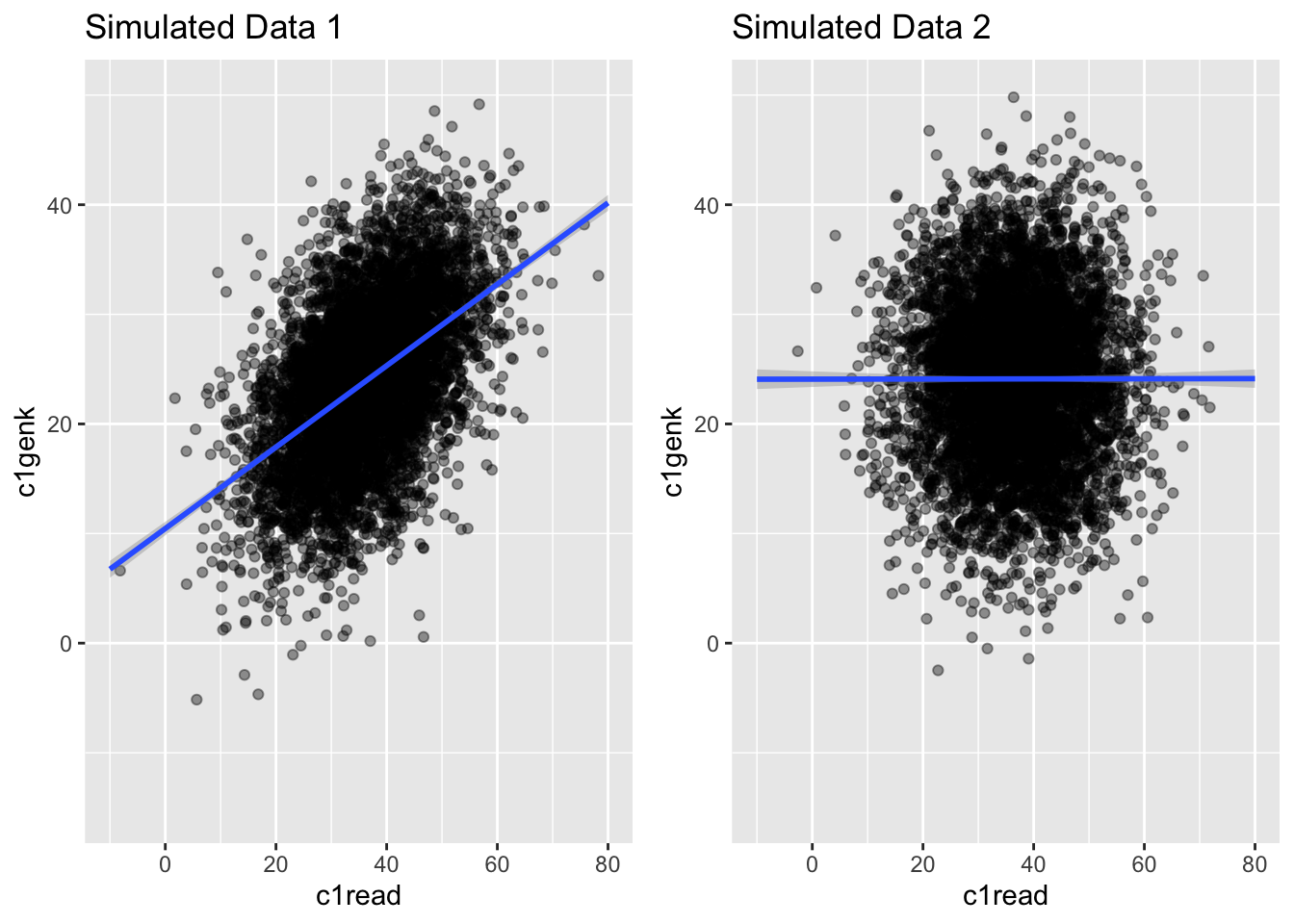
8.13 Comparing Models
mod1 <- lm(c5read ~ c1read, data = simach3orthogonal)
mod2 <- update(mod1, . ~ c1genk)
mod3 <- update(mod1, . ~ . + c1genk)
mod4 <- lm(c5read ~ c1read + c1genk, data = simach3)
htmlreg(list(mod1, mod2, mod3, mod4), doctype = FALSE)| Model 1 | Model 2 | Model 3 | Model 4 | |
|---|---|---|---|---|
| (Intercept) | 81.27*** | 82.89*** | 30.19*** | 63.64*** |
| (1.09) | (0.90) | (0.99) | (1.04) | |
| c1read | 1.44*** | 1.44*** | 0.84*** | |
| (0.03) | (0.02) | (0.03) | ||
| c1genk | 2.12*** | 2.12*** | 1.61*** | |
| (0.04) | (0.03) | (0.04) | ||
| R2 | 0.29 | 0.36 | 0.65 | 0.44 |
| Adj. R2 | 0.29 | 0.36 | 0.65 | 0.44 |
| Num. obs. | 6206 | 6206 | 6206 | 6206 |
| ***p < 0.001; **p < 0.01; *p < 0.05 | ||||
9 Issues in Multiple Regression
# Matrix A from Table 1 of Gordon (1968, p. 597)
matrixA <- matrix(c(1.0, 0.8, 0.8, 0.2, 0.2, 0.6,
                    0.8, 1.0, 0.8, 0.2, 0.2, 0.6,
                    0.8, 0.8, 1.0, 0.2, 0.2, 0.6,
                    0.2, 0.2, 0.2, 1.0, 0.8, 0.6,
                    0.2, 0.2, 0.2, 0.8, 1.0, 0.6,
                    0.6, 0.6, 0.6, 0.6, 0.6, 1.0),
nrow = 6)kable(matrixA)| 1.0 | 0.8 | 0.8 | 0.2 | 0.2 | 0.6 |
| 0.8 | 1.0 | 0.8 | 0.2 | 0.2 | 0.6 |
| 0.8 | 0.8 | 1.0 | 0.2 | 0.2 | 0.6 |
| 0.2 | 0.2 | 0.2 | 1.0 | 0.8 | 0.6 |
| 0.2 | 0.2 | 0.2 | 0.8 | 1.0 | 0.6 |
| 0.6 | 0.6 | 0.6 | 0.6 | 0.6 | 1.0 |
matrixB <- matrix(
  c(1.0, 0.8, 0.8, 0.8, 0.2, 0.2, 0.2, 0.2,
    0.8, 1.0, 0.8, 0.8, 0.2, 0.2, 0.2, 0.2,
    0.8, 0.8, 1.0, 0.8, 0.2, 0.2, 0.2, 0.2,
    0.8, 0.8, 0.8, 1.0, 0.2, 0.2, 0.2, 0.2,
    0.2, 0.2, 0.2, 0.2, 1.0, 0.8, 0.8, 0.2,
    0.2, 0.2, 0.2, 0.2, 0.8, 1.0, 0.8, 0.2,
    0.2, 0.2, 0.2, 0.2, 0.8, 0.8, 1.0, 0.2,
    0.2, 0.2, 0.2, 0.2, 0.2, 0.2, 0.2, 1.0),
  nrow = 8)
matrixC <- matrix(
c(1.0, 0.8, 0.8, 0.8, 0.2, 0.2, 0.2, 0.2, 0.6,
0.8, 1.0, 0.8, 0.8, 0.2, 0.2, 0.2, 0.2, 0.6,
0.8, 0.8, 1.0, 0.8, 0.2, 0.2, 0.2, 0.2, 0.6,
0.8, 0.8, 0.8, 1.0, 0.2, 0.2, 0.2, 0.2, 0.6,
0.2, 0.2, 0.2, 0.2, 1.0, 0.8, 0.8, 0.2, 0.6,
0.2, 0.2, 0.2, 0.2, 0.8, 1.0, 0.8, 0.2, 0.6,
0.2, 0.2, 0.2, 0.2, 0.8, 0.8, 1.0, 0.2, 0.6,
0.2, 0.2, 0.2, 0.2, 0.2, 0.2, 0.2, 1.0, 0.6,
0.6, 0.6, 0.6, 0.6, 0.6, 0.6, 0.6, 0.6, 1.0),
nrow = 9)